The return-period model
This section documents the model that predicts how often earthquakes,
and shaking at the site, recur. It is a screening-level PSHA in the
tradition of Cornell (1968), with a gridded background source and a
separate fault source, implemented in the function
run_forecast of the analysis script (Section [sec:repro]).
Definitions and the Poisson
assumption
Earthquakes are assumed to occur as a Poisson process: independent,
with constant average rate
per year. The probability of at least one event in
years is then
and the return period is
.
For a ground-motion level
,
is the annual rate of exceeding
at the site, and the PGA with return period
is the
satisfying
.
A 475-year return period corresponds to a 10% chance of exceedance in 50
years and 2,475 years to 2%. Because earthquakes cluster, the Poisson
model is applied only to declustered mainshocks. A return period of
ground motion is the reciprocal of an exceedance rate; it is
not the recurrence interval of any particular earthquake.
Source zone and
declustering
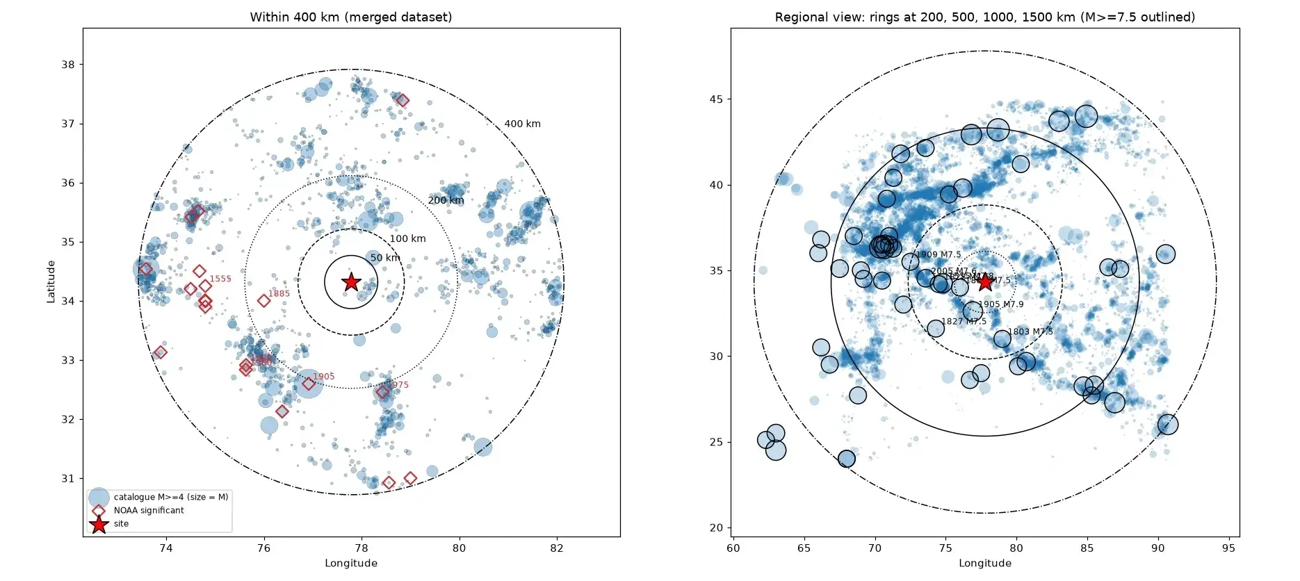
The background source zone is the disc of radius 400 km around the
site (the limit of the ground-motion model). To avoid edge effects,
declustering and smoothing use events out to 550 km. Since 1902 there
are 1,631 events inside the zone. Foreshocks and aftershocks were
removed with the windows of Gardner and Knopoff (1974): a smaller event
is dropped if it lies within the distance
and time
of a larger one,
applied
in time and processed from the largest event downward. Of the 1,631
events, 814 (50%) remain as mainshocks. For
M4.5,
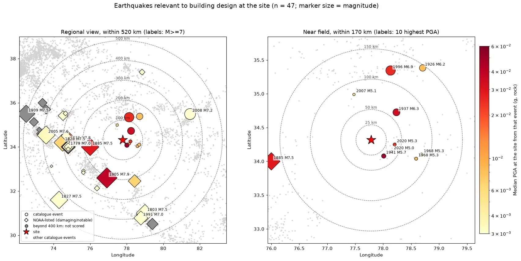
483 of 890 are kept (Figure 4, right). Rate
estimation, the back-test and the spatial smoothing use
catalogue-sourced events only: the NOAA records are a selected subset.
One NOAA-only mainshock lies inside the zone (1963, M5.3, 279 km); it
falls before its magnitude bin’s completeness year, so excluding it
changes nothing.
Magnitude-dependent
completeness
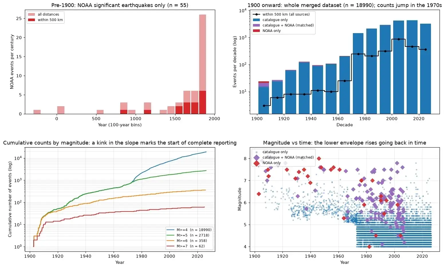
Completeness years by 0.5-unit magnitude bin were read from the
decade counts and cumulative curves of the merged data:
| Bin lower edge |
4.0 |
4.5 |
5.0 |
5.5 |
6.0 |
6.5 |
| Complete from |
excluded |
1973 |
1964 |
1930 |
1904 |
1902 |
The M4.0–4.5 bin is excluded because its observed rate is lower than
that of the M4.5–5.0 bin, which can only mean incomplete reporting in
this remote region. Including it flattens the fitted
-value
to 0.78 and produces an implausible
M6
return period of 3 years. The completeness table can be overridden with
–completeness.
Gutenberg–Richter recurrence by
maximum likelihood
Magnitudes are assumed to follow the Gutenberg–Richter law (Gutenberg
and Richter, 1944),
,
equivalently an exponential distribution with
.
Because each bin has its own observation period, the parameters are
estimated by the maximum-likelihood method of Weichert (1980). In bin
with edges
,
observed for
years with
mainshocks, the expected rate is
and the Poisson log-likelihood is
.
Maximizing over
gives
with
,
leaving a profile likelihood in
only,
which is maximized on a fine grid. The standard error is
from the numerical curvature.
Result (476 mainshocks):
.
The annual rates inside the 400 km zone are 2.18 events/yr for
,
0.158/yr for
(return period 6.3 years) and 0.0115/yr for
(return period 87 years). The standard error is statistical only,
conditional on the catalogue, the completeness table and the magnitudes
as given; it excludes uncertainty from magnitude type (in the fit window
310 of 319 events in M4.5–5.0 and 58 of 105 in M5.0–5.5 are mb), event
selection and completeness (Section 8.7). Table 4
compares fitted and observed counts.
Recurrence fit: observed and expected mainshock counts within
400 km in each bin’s completeness window, with two-sided Poisson
-values
(computed from unrounded expected counts).
| M4.5–5.0 |
53 |
319 |
315.9 |
0.87 |
| M5.0–5.5 |
62 |
105 |
99.4 |
0.60 |
| M5.5–6.0 |
96 |
26 |
41.4 |
0.01 |
| M6.0–6.5 |
122 |
19 |
14.2 |
0.25 |
| M6.5–7.0 |
124 |
4 |
3.9 |
1.00 |
| M7.0–7.5 |
124 |
1 |
1.0 |
1.00 |
| M7.5–8.0 |
124 |
2 |
0.3 |
0.07 |
Goodness of fit. The fit is in-sample, so these
tests are generous. The largest bin stands out: two M7.5–8.0 mainshocks
(presumably the 1905 Kangra and 2005 Kashmir earthquakes) were observed
against 0.3 expected, about seven times the expectation; the probability
of two or more under a Poisson model with mean 0.28 is 3.3% (one-sided),
or 0.07 on the two-sided scale used in the table. With seven bins, one
such value is not surprising, and magnitude scales in the catalogue are
heterogeneous and the sample is tiny, so it is a warning and not proof
of misfit. Pooling all
M6.5
gives 7 observed against about 5.2 expected
(),
no evidence of misfit for the pooled tail. The M5.5–6.0 bin (26 against
41,
)
is the clearest individual misfit and probably reflects completeness or
magnitude-conversion problems rather than physics. The magnitude types
support the second reading: the M5.5–6.0 bin is 23 of 26 moment-type,
whereas the bins that dominate the
-value
are mostly mb, so the deficit appears on a different magnitude scale
from the one that sets the slope. Together with the clustering of the
largest events, this is a reason to investigate magnitude homogenisation
and source zonation (Section 10), not a
minor statistical detail; Section 8.7 shows how
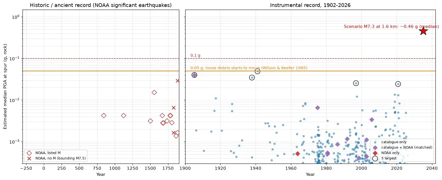
much the result moves. The practical effect on the site is small: an
M7.9 event 150 km away gives only about 0.03 g at the site, and above a
few hundred years the hazard is controlled by the fault, not the
background.
Hazard magnitude bins and
maximum magnitude
For the hazard integral the recurrence law is evaluated in 0.1-unit
bins from M4.5 (smaller events are not damaging) up to a maximum
magnitude
:
Rates in the observed magnitude range are therefore unchanged by the
choice of
,
which only removes the tail.
is a logic-tree branch (7.5, 7.9, 8.3 with weights 0.3, 0.5, 0.2). The
largest catalogue magnitude within 400 km is the M7.9 Kangra earthquake
of 1905, so any branch below it contradicts the catalogue: every
branch below the largest catalogue magnitude within 400 km is
raised to it and the weights of merged branches are added (events with
an assumed magnitude, such as the 1885 Kashmir M7.5, do not set the
floor). The branches become 7.9 (weight 0.8) and 8.3 (weight 0.2). The
floor has little effect on shaking at the site, because it only adds
rate to M7.5–7.9 events that are typically more than 150 km away. Kangra
is M7.9 in both data files; some compilations give
7.8,
which would move the floor by 0.1 unit and, by the same argument, matter
little.
Spatial distribution: smoothed
seismicity
The zone is a grid of 5,025 cells of
km.
The share
of the zone’s seismicity assigned to cell
is obtained by Gaussian smoothing (as in Frankel, 1995) of the
declustered
M4.5
mainshocks,
where
is the distance from cell
to event
,
is the completeness year for the event’s magnitude (so each event counts
as the annual rate it represents) and
km
(option –smooth-km). The rate of magnitude bin
in cell
is
.
Quiet surroundings mean that only 0.8% of the zone’s rate falls within
50 km of the site, 3.5% within 100 km and 22.6% within 200 km. Each
cell’s source distance is
,
so a cell on top of the site is not at zero distance; this term accounts
for the spread of sources within a cell and is not a source depth
(Section 4).
The Karakoram Fault source
The background catalogue contains no large events on the fault, so
the fault is modelled separately as a characteristic-earthquake source
at
km.
The rate is set by the slip budget, not the catalogue. A point on the
fault must slip on average
in every characteristic rupture, with (Wells and Coppersmith, 1994)
metres, giving 0.95 m for M7.0, 1.78 m for M7.3, 3.31 m for M7.6 and
4.07 m for M7.7. The annual rate is
where
is the slip rate and
the coupling, the fraction of slip released seismically (default
,
the conservative choice; option –coupling). Slip-budget
recurrence intervals
are (years):
| M7.0 |
955 |
477 |
318 |
239 |
| M7.3 |
1,778 |
889 |
593 |
445 |
| M7.6 |
3,311 |
1,656 |
1,104 |
828 |
| M7.7 |
4,074 |
2,037 |
1,358 |
1,018 |
These are conditional on the fault being active, and are slip-budget
estimates, not observed recurrence intervals. The characteristic
magnitudes are alternative descriptions of the same fault, not
events to be added together. Weighting the branches below, the mean
characteristic-earthquake rate is about 0.0011 per year (mean return
period about 900 years): about 0.0015 per year (650 years) under
hypothesis A and 0.0003 per year (3,100 years) under hypothesis B. These
derived figures depend entirely on the assumed slip rates and coupling,
and on the assumption that every characteristic rupture releases the
average slip at the site-adjacent reach; they are the model’s largest
single uncertainty.
Evidence for fault slip at the
site
The slip-rate range is taken from published geodetic and geological
studies of the Karakoram Fault, summarised in Table 5.
Published constraints on Karakoram Fault slip relevant to the
Agham reach.
| Mohanty et al. (2024) |
Continuous GPS over more than 300 km:
Nubra valley (K2 segment of the northern fault) inactive;
Bangong–Chaxikang (southern fault) 1.6–3.2 mm/yr, on the Pangong strand;
the Tangtse strand takes no slip. |
Nine-year GPS snapshot; applies to the
strands crossed by its profiles, not shown to include the trace 1.6 km
from the site. |
| Wang et al. (2026) |
GNSS and InSAR block model: northern
segment (about 36.2–37°N) can be below 1 mm/yr; the middle and southern
segments (about 30.5–35°N) are faster. |
Regional model rate. The authors warn that
strong coupling on the Main Frontal Thrust may bias the inferred rate
and that it may not equal the long-term rate. |
| Brown et al. (2002) |
mm/yr
from cosmogenic dating of offset debris flows and moraines in
Ladakh. |
A geological rate for another reach (the
Tangtse Valley study area); the basis of the 4 mm/yr upper branch, not a
measurement at the site and not transferable to the assumed strand
without evidence. |
| Bohon et al. (2010) |
A Quaternary strand in the Tangyar valley
with offset alluvial surfaces; slip rate undetermined at the time. |
Shows that a possibly active parallel
strand exists in the sector; not shown to be the trace at the site. |
| Ojha (2026) |
Segmented, “stop-and-go” behaviour; last
kinematic readjustment about 0.5 Ma. |
A structural age, not a dated last rupture
and not a recurrence interval. |
| Wang and Shen (2020) |
Continental GPS model: northern segment
about 0, southern about 3 mm/yr. |
Not independent of the GPS data used in
other analyses; not a second confirmation. |
The site (34.32°N) falls in the latitude band of the faster middle
and southern segments of Wang et al., but lies within the Nubra sector,
where the inactive result of Mohanty et al. applies. Which strand lies
1.6 km from the site, and whether it is the inactive Nubra/K2 strand, an
active parallel Quaternary strand, or a distinct reach, is not settled
by the published literature at coordinate level. For that reason the
model keeps both outcomes open instead of selecting one slip rate
(Sections 7.10 and 7.11). The
weights placed on the alternatives are analyst judgement, not quantities
established by the literature.
The hazard integral
Given a median PGA
from Section 4, the probability that a
magnitude-
event at distance
exceeds
at the site, with scatter truncated at
,
is
with
the standard normal distribution function and
the BSSA14 standard deviation of Section 4. The two-sided
truncation requires the normalising constant
and clamping
at both ends, so that
when
is more than
below the median and
when it is more than
above. The annual rate of exceeding
for one logic-tree branch is the sum of the background and fault
contributions,
Median PGAs are tabulated on a distance grid and interpolated, which is
exact for the embedded model and fast enough for pygmm. The
level
runs over 70 values from 0.005 to 2 g.
Logic tree
Uncertain parameters are combined as independent branches with
weights:
|
(b-value) |
|
0.25, 0.5, 0.25 |
| Background
(floored at the largest observed magnitude) |
7.9, 8.3 |
0.8, 0.2 |
| Fault slip rate (mm/yr) |
0, 1, 2, 3, 4 |
0.15, 0.20, 0.30, 0.25, 0.10 |
| Characteristic magnitude |
7.0, 7.3, 7.6, 7.7 |
0.25, 0.35, 0.25, 0.15 |
This gives
branches. The mean hazard is the weighted mean of the branch rates,
.
The 16th and 84th percentiles are weighted quantiles of the branch
exceedance rates
at each
(percentile curves), and the tabulated 16% and 84% PGAs come
from inverting those curves at
.
These bands are epistemic: they show spread among logic-tree
branches, not the scatter of one earthquake’s ground motion, which is
the aleatory
already inside every branch curve. Where branch curves cross, this is
not the same as inverting each branch first and taking weighted
percentiles of the branch PGAs; the script computes that version as a
cross-check, and here the two agree to within 0.00014 g at every
tabulated return period. The return-period PGA
is found by log–log interpolation of
at
.
The slip-rate and magnitude weights are judgements, not measurements;
the weight of 0.15 on zero slip and the weights on the M7.6 and M7.7
branches in particular are analyst choices. The next subsection shows
how results are reported so that they do not depend on them.
Fault-activity hypotheses and
the governing envelope
The slip-rate branches fall into two explicit hypotheses:
A, the fault slips at a rate consistent with the
geodetic and geological studies of the active segments (2, 3, 4 mm/yr;
tree weight 0.65) and B, inactive or very low (0,
1 mm/yr; tree weight 0.35). Within each hypothesis the branch weights
are renormalised and the mean hazard
,
is computed with the background and magnitude branches unchanged. The
governing envelope is
at each
.
The 0.65/0.35 split is a judgement; the conditional curves and the
envelope do not depend on it. These are conditional curves, not
predictions: the model does not say which hypothesis is true. The
envelope is conservative only relative to A and B; it does not cover the
ground-motion-model, site-response, rupture-geometry or catalogue
uncertainties listed in Section 10.
Forecasting earthquakes and
shaking in the building’s life
Using the mean rates, the rate of earthquakes of magnitude at least
within radius
is
where the last term adds characteristic fault events when they qualify.
The probability of at least one in
years is then
.
The probability that PGA at the site exceeds
in
years is
.
A 475-year return period is a statistical measure of how often shaking
of that size is exceeded under a Poisson model; it does not mean that an
earthquake occurs every 475 years or that the next one is 475 years
away.
Disaggregation
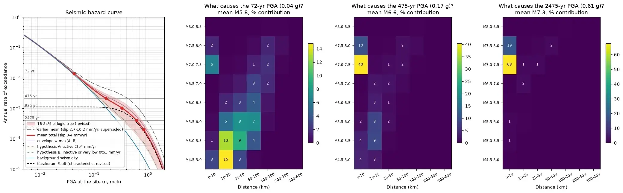
To identify the controlling earthquakes, the mean-model contribution
to
was split into magnitude bins (0.5 wide) and distance bins (0–10, 10–25,
25–50, 50–100, 100–200, 200–300, 300–400 km). Fault events are placed in
the 0–10 km bin, and the fault source is also tracked separately so that
it can be told apart from background earthquakes that happen to lie
within 10 km.
Back-test
A split-sample back-test fitted the recurrence model to mainshocks
before 2000
()
and compared predicted with observed counts for 2000–2026 (Table 6). Two-sided Poisson
-values
are given. The sparse M6.5–7.0 and M7.0–7.5 bins are statistically
uninformative.
Back-test of the background recurrence model,
2000–2026.
| M4.5–5.0 |
144.4 |
167 |
0.07 |
| M5.0–5.5 |
40.0 |
51 |
0.11 |
| M5.5–6.0 |
11.1 |
5 |
0.07 |
| M6.0–6.5 |
3.1 |
3 |
1.00 |
| M6.5–7.0 |
0.9 |
0 |
0.85 |
| M7.0–7.5 |
0.2 |
1 |
0.42 |
The model predicts counts of the right order in every bin and no bin
is rejected at the 5% level. There is a pattern: more M4.5–5.5 events
than predicted and fewer M5.5–6.0, consistent with a shift in the
catalogue’s magnitude scale after about 2000, as moment magnitudes
replaced mb for mid-sized events. The back-test tests the background
source only; the fault source cannot be tested against a record that
contains no large fault earthquake.